FAQ Page #

Please use our common issues and frequently asked questions page as a resource. We’ll be updating this FAQ page on the website throughout the week! In future labs, we’ll link the FAQ at the top.

Introduction #

Different data structures perform differently in different situations. In this lab, we’ll explore a couple of these situations for the AList and SLList classes we discussed in lecture.

Setup #

Follow the assignment workflow instructions to get the assignment and open it in IntelliJ. This assignment is lab03.

Goals and Outcomes #

In this lab, you will solidify your understanding of why we have different kinds of data structures by analyzing the time they take to perform certain operations.

By the end of this lab, you will…

• Understand that different data structures have different time guarantees.
• Be able to empirically measure the runtime of a program.
• Interpret timing experiments and reason about their implications.

Lab 2 Part 2: Adventure #

First, head back to Lab 02 to complete the Adventure section of the lab! In this section, you’ll see some common Java errors. For this week, we have already fixed BeeCountingStage for you.

Timing Experiments #

Overview #

You learned in 61A how to construct correct solutions to problems, but didn’t worry too much about how fast they run. One way of determining the speed of a given program is to test it on a variety of inputs and measure the time it takes for each one. This is called a timing experiment, and we refer to this process as finding the efficiency of a program empirically. In this lab, we will be doing some timing experiments to see how the AList and SLList classes we discussed in lecture perform.

We’ll learn more about how to theoretically formalize this notion of “speed” later in 61B, but for now, we’ll stick to empirical methods.

In this part of the lab, we will be working with the code in the timing package.

TimingData #

In a timing experiment, we are interested in seeing how the time of some operations scales with the size of the computation. The output of a timing experiment will be an instance of the following class:

public class TimingData {
    private List<Integer> Ns;
    private List<Double> times;
    private List<Integer> opCounts;
    // Some utility methods for accessing data
}

In this class, we have three parallel lists, storing data from a bunch of trials. The data for trial i is stored at index i in each list:

Ns

The size of the data structure, or how many elements it contains.

times

The total time required for all operations, in seconds.

opCounts

The number of operations made during the experiment. For example, we might do many operations to take an average over.

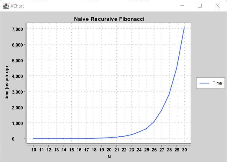
Example: Fibonacci #

As an example, let’s look at timing a method that computes the N-th Fibonacci number, very inefficiently. Open the timing/Experiments.java file, and look at the fib and exampleFibonacciExperiment.

The most interesting part is the for loop in the experiment:

for (int N = 10; N < 31; N++) {
    Ns.add(N);
    opCounts.add(ops);
    Stopwatch sw = new Stopwatch();
    for (int j = 0; j < ops; j++) {
        int fib = fib(N);
    }
    times.add(sw.elapsedTime());
}

1. We compute the 10th through 30th Fibonacci numbers in the outer loop. This is our computation “size”, so we add it to the Ns list. (For small N, fib is quite fast and will probably be subject to machine noise.)
2. We also do this computation 100 times to collect a lot of samples and make sure we get a good average time, so we add 100 to the opCounts list.
3. To time code, we use Princeton’s Stopwatch class. We construct a Stopwatch just before the code we want to time, and call stopwatch.elapsedTime() at the end to see how much time has passed in seconds. This time is added to the times list.
4. Inside the inner for loop, we simply call the fib function ops times on the argument N. This for loop is timed.

Note that all 3 lists have the same length.

Timing Tables #

One way that we could look at the collected data is by printing the lists in a table:

           N     time (s)        # ops  microsec/op
------------------------------------------------------------
          10         0.00          100         0.00
          11         0.00          100         0.00
          12         0.00          100        10.00
          13         0.00          100         0.00
          14         0.00          100         0.00
          15         0.00          100        10.00
          16         0.00          100        10.00
          17         0.00          100        10.00
          18         0.00          100        20.00
          19         0.00          100        40.00
          20         0.01          100        60.00
          21         0.01          100       100.00
          22         0.02          100       150.00
          23         0.03          100       250.00
          24         0.04          100       420.00
          25         0.06          100       630.00
          26         0.11          100      1070.00
          27         0.18          100      1810.00
          28         0.28          100      2830.00
          29         0.45          100      4510.00
          30         0.71          100      7080.00

The first 3 columns are the data we collected and described above. The last column, as its header says, is the number of microseconds it took on average to perform each operation. Here, an “operation” is a call to fib(N). Note that ops is always the same here, because we were timing the same number of calls every time.

Here are some things to notice about the above table:

• fib(N) takes longer to compute when N is larger. Many functions will take a longer time to complete when the input or underlying data is larger.

• For 15, 16, 17, and others, the time per fib(N) calll is the same, despite being different numbers. For small inputs, timing results are not precise for two reasons:

  • The variance in runtime is high, for reasons beyond the scope of the course (and covered in CS 61C).
  • The accuracy of our System clock (milliseconds) is insufficient to resolve the difference between runtimes for these calls.

  This can also lead to strange situations, such as the runtime for 12 being larger than the runtime for 13. Therefore, when we use empirical timing tests, we focus on the behavior for large N – note that the differences are much larger, and easier to distinguish!

Finally, the times that you get may be very different from the table that’s written above. That’s okay, as long as the general trend is the same. In 61C, you will learn exactly why the same code may take vastly different amounts of time on different hardware. In 61B (and in most theory-based classes) we are only concerned with general trends, which hide parts of reality that are hard to account for. While reasoning about “general trends” may seem tricky, we will learn a formalism for this later in the course (asymptotics). For now, use your intuition!

Plots #

While we can do some things with numbers, it’s hard to really feel the “order of growth” in a text table. We can also use a graphing library to generate plots!

AList, Bad Resizing #

As discussed in lecture, a multiplicative resizing strategy will result in fast add operations (good performance), while an additive resizing strategy will result in slow add operations (bad performance). In this part of the lab, we’ll put visuals to these statements!

In the timing package, we’ve provided the AList class created in lecture with the bad resizing strategy below:

public void addLast(Item x) {
    if (size == items.length) {
        resize(size + 1);
    }

    items[size] = x;
    size = size + 1;
}

In this part of the lab, you’ll write code that tabulates the amount of time needed to create a AList of various sizes using the addLast method above.

• N should take on the values of 1000, 2000, all the way to 128000, doubling each time.
• You should time the entire time it takes to construct an AList of size N from scratch. That is, you will need a new AList for each value of N, and you will have an inner for loop containing a call to addLast.
• We’re interested in the average time per addLast call, so the number of operations is the number of addLast calls, or N.

Note: If your computer is a little slow, you might want to stop at 64000 instead of 128000.

AList, Good Resizing #

Your AList objects should now be constructed nearly instantly, even for N = 128000, and each add operation should only take a fraction of a microsecond. You might observe some strange spikes for “small” N – these are due to, again, 61C material.

Optional: Try increasing the maximum N to larger values, e.g. 10 million. You should see that the time per add operation remains constant.

Optional: Try experimenting with different resizing factors and see how the runtimes change. For example, if you resize by a factor of 1.01, you should still get constant time addLast operations! Note that to use a non-integer factor you’ll need to convert to an integer. For example, you can use Math.round().

public void addLast(Item x) {
    if (size == items.length) {
        resize((int) (size * 1.01));
    }

    items[size] = x;
    size = size + 1;
}

SLList.getLast #

Above, we showed how we can time the construction of a data structure. However, sometimes we’re interested in the dependence of the runtime of a method on the size of an existing data structure that has already been constructed.

For example, in your LinkedListDeque, you are supposed to have addLast operations that are fast… a single addLast operation must take “constant time”, i.e. execution time should not depend on the size of the deque.

In this part of the lab, we’ll show you how to empirically test whether a method’s runtime depends on the size of the data structure.

Suppose we want to compute the time per operation for getLast for an SLList and want to know how this runtime depends on N. To do this, we need to follow the procedure below:

1. Create an SLList.
2. Add N items to the SLList, for N from 1000 through 128000 and doubling.
3. Start the timer.
4. Perform M getLast operations on the SLList.
5. Check the timer. This gives the total time to complete all M operations.

It’s important that we do not start the timer until after step 2 has been completed. Otherwise the timing test includes the runtime to build the data structure, whereas we’re only interested how the runtime for getLast depends on the size of the SLList.

Note that the N and # ops columns are not the same. This is because we are always calling getLast the same number of times regardless of the size of the list, i.e. M = 10000 for step 4 of the procedure described above.

Secondly, the operations are again not constant time! (If your results imply that the operations are constant time, make sure you’re running your tests on the SLList instead of the AList!). This means that as the list gets bigger, the getLast operation becomes slower. This would be a serious problem in a real world application. For example, suppose the list is of ATM transactions, and the getLast operation was being called in order to get the most recent transaction to print a receipt. Every time the ATM is used, the next receipt would take a little bit longer to print. Eventually over many months or years, the list would become so large that the getLast operation would be unusably slow. While this is a contrived example, similar problems have plagued real world systems!

For this reason, the LinkedListDeque that you build in Project 1A will be required to have a runtime that is independent of the size of the data structure. In other words, the last column will be some approximately constant value.

Optional: Try running a timing test for getting the last element of a Java LinkedList, with list.get(list.size() - 1). What do you think it does to achieve this?

Optional question to ponder: Why is getLast so slow? What is special about your LinkedListDeque that makes the getLast function faster?

Deliverables and Scoring #

The lab is out of 256 points. There are no hidden tests on Gradescope. If you pass all the local tests, you will receive full credit on the lab.

• The remaining adventure stages in your lab03/adventure directory. (BeeCountingStage is already done for you.)
  • SpeciesListStage (32 pts)
  • PalindromeStage (32 pts)
  • MachineStage (32 pts)
  • Integration test for the entire game (32 pts)
• timing/Experiments.java
  • timeAListConstruction (64 pts)
  • timeSLListGetLast (64 pts)

Submission #

Just as you did for the previous assignments, add, commit, then push your Lab 3 code to GitHub. Then, submit to Gradescope to test your code. If you need a refresher, check out the instructions in the Lab 1 spec and the Assignment Workflow Guide.